3 Working with Graphs in Main Memory
3.1 Data Structures
Graph data can be represented in main memory in several different ways. This section aims to give an overview of the characteristics, advantages, and shortcomings of the four most important main memory graph data structures: the unordered edge list, the compressed storage format (CSR), adjacency lists, and the adjacency matrix.
The CSR is the main graph data structure in G-Store. The unordered edge list data structure is important for the discussion of relational database graph data structures in Section 4.1. Adjacency lists and adjacency matrix are the two most common graph data structures in practice.
To simplify the discussion, we assume in
this section that vertices are uniquely identified by integers in the range ![]() . We use
. We use ![]() informally to denote this range, and
informally to denote this range, and ![]() and
and ![]() to denote integers in the interval.
to denote integers in the interval.
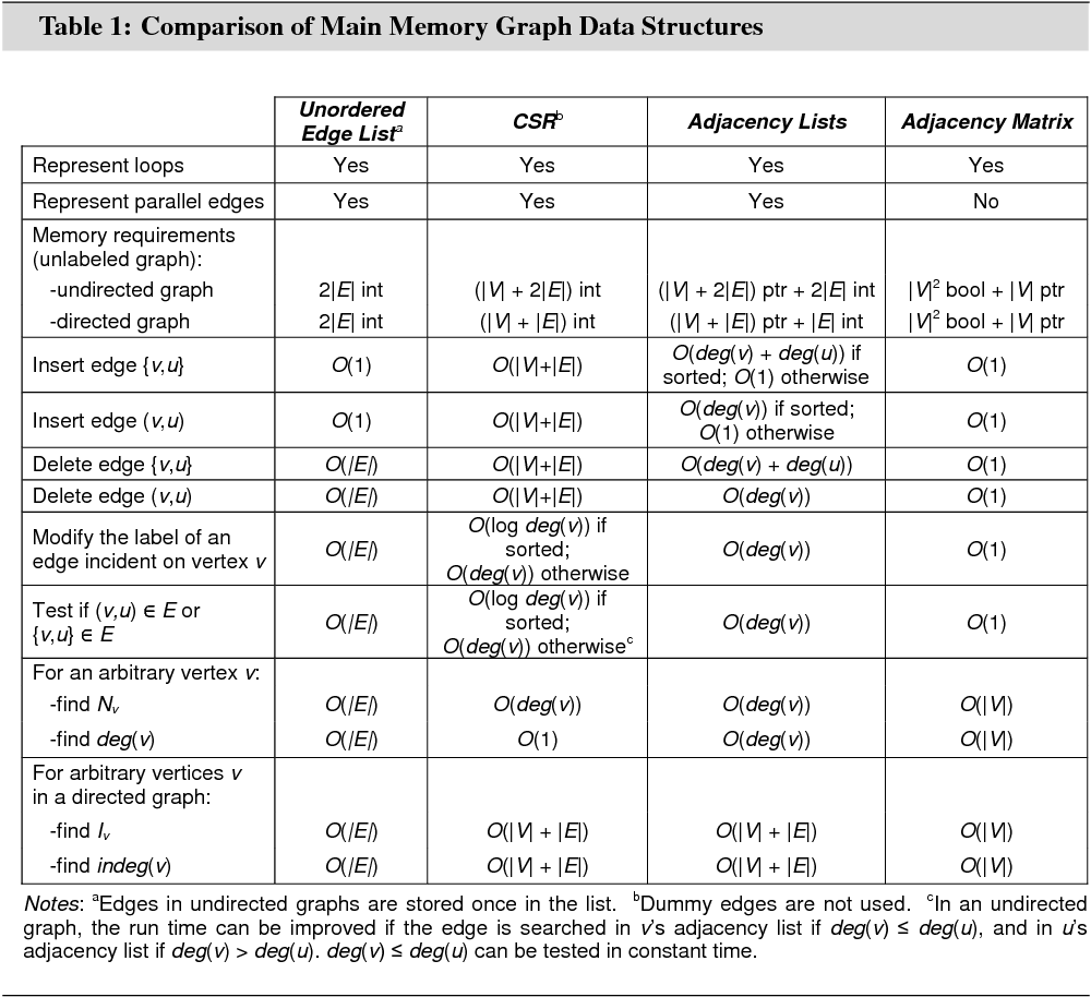
Figures 3 and 4 illustrate the different data structures for an undirected graph and an edge-weighted directed graph. Table 1 summarizes the memory requirements and algorithmic properties of the data structures.
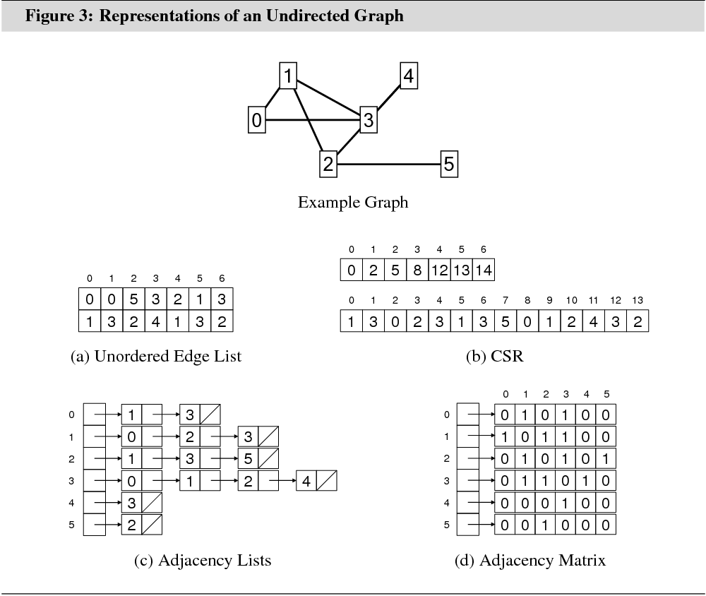
3.1.1 Unordered Edge List
The simplest way to represent a graph in main memory is as an unordered list of edges. This structure uses only a single two-column array, such as generated in C++ by:
struct edges{ int a; int b;};std::vector<edges> edgelist;
The two-column structure naturally imposes an order on the two vertices in an edge. This is useful for representing directed graphs: The first column can be taken to hold the source of each edge, and the second column can be taken to hold the destination of each edge.
There are two solutions for dealing with
the imposed order for undirected graphs: Ignoring it, or including each edge ![]() twice in the edge list, once as
twice in the edge list, once as ![]() and once as
and once as ![]() .
With the former solution, many algorithms that have been designed for directed
graphs will not work properly anymore. An application that should support
directed and undirected graphs must implement two versions of several
algorithms. The latter solution creates redundancy and increases the cost of
modifying the edge list.
.
With the former solution, many algorithms that have been designed for directed
graphs will not work properly anymore. An application that should support
directed and undirected graphs must implement two versions of several
algorithms. The latter solution creates redundancy and increases the cost of
modifying the edge list.
If existent, edge labels can be stored either as part of struct edges or in an additional array that copies the order of edges in the edge list. If several edges have the same labels, storing labels in an external data structure, referenced by pointers from the edge list may be considered.
Inserting an arbitrary edge into the edge
list takes amortized constant time (i.e., constant time if the cost of resizing
the array is ignored). Finding all vertices in ![]() for
a given vertex
for
a given vertex ![]() , or
testing whether a particular edge exists in
, or
testing whether a particular edge exists in ![]() , on the other hand, takes time
, on the other hand, takes time ![]() , which is forbiddingly slow.
, which is forbiddingly slow.
With 4 bytes per integer, storing an unlabeled directed graph with 1 million vertices and 15 million edges in an unordered edge list uses at least 114.44 MB of main memory.
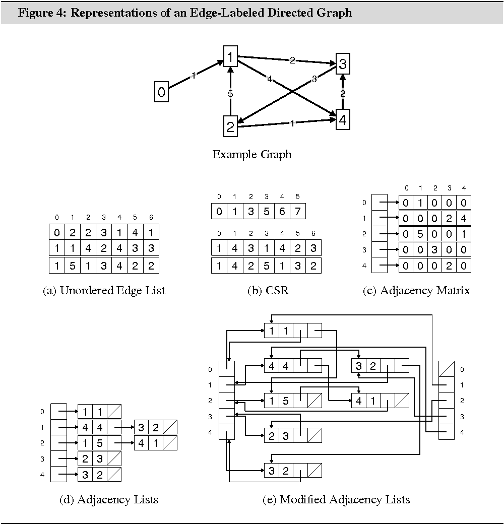
3.1.2 Compressed Storage Format
The compressed storage format (CSR) is most effective for storing static sparse graphs. It uses memory efficiently and has good algorithmic properties, except for operations that modify the graph. It uses two arrays, such as generated by the following C++ code:
std::vector<int> offset_e, e_to;
e_to stores adjacency lists for all vertices. The adjacency list
for an arbitrary vertex stores all vertices in the neighborhood of that vertex.
offset_e stores offsets into e_to that indicate where the
adjacency lists begin. The list for an arbitrary vertex ![]() begins at e_to[offset_e[v]] and ends at e_to[offset_e[v+1]]-1. Array offset_e has size
begins at e_to[offset_e[v]] and ends at e_to[offset_e[v+1]]-1. Array offset_e has size ![]() and array e_to has size
and array e_to has size ![]() for directed graphs, and
size
for directed graphs, and
size ![]() for undirected graphs.
for undirected graphs.
If existent, edge labels are stored in an additional array that copies the order of edges in e_to.
The CSR has several advantages over
standard adjacency lists (introduced in the next section). For instance, the
degree of vertex ![]() can be
determined in constant time by subtracting offset_e[v] from offset_e[v+1]. With standard adjacency lists,
this takes time
can be
determined in constant time by subtracting offset_e[v] from offset_e[v+1]. With standard adjacency lists,
this takes time ![]() .
.
Moreover, if we sort the adjacency lists,
we can use binary search to determine in time ![]() if
a particular edge incident on vertex
if
a particular edge incident on vertex ![]() is part of the graph. With standard adjacency
lists, this takes time
is part of the graph. With standard adjacency
lists, this takes time ![]() .
.
On the other hand, modifying the graph is
prohibitively expensive. Inserting an edge ![]() requires
shifting the entire array e_to between e_to[offset_e[v]] and e_to[offset_e[|V|+1]] right by one position,
and updating offset_e between v+1 and |V|+1.
Deleting an edge has the same complexity.
requires
shifting the entire array e_to between e_to[offset_e[v]] and e_to[offset_e[|V|+1]] right by one position,
and updating offset_e between v+1 and |V|+1.
Deleting an edge has the same complexity.
A technique to speed up edge insertion and
deletion is the inclusion of dummy edges in e_to. A
dummy edge is a special integer that represents deleted or otherwise
non-existent edges. With dummy edges, deleting an edge takes only time ![]() for unsorted adjacency lists, and time
for unsorted adjacency lists, and time
![]() for sorted adjacency lists. Inserting
an edge still takes time
for sorted adjacency lists. Inserting
an edge still takes time ![]() in the worst case.
However, if e_to contains enough dummy edges, the average insertion time will be
much lower. On the downside, dummy edges clutter up e_to and
slow down other graph operations. Moreover, subtracting offset_e[v] from offset_e[v+1] no longer yields the degree of
in the worst case.
However, if e_to contains enough dummy edges, the average insertion time will be
much lower. On the downside, dummy edges clutter up e_to and
slow down other graph operations. Moreover, subtracting offset_e[v] from offset_e[v+1] no longer yields the degree of ![]() .
.
With 4 bytes per integer, storing an unlabeled directed graph with 1 million vertices and 15 million edges in the CSR uses at least 61.04 MB of memory. This is the lowest value among the data structures compared.
3.1.3 Adjacency Lists
This is perhaps the most commonly used main memory data structure for graphs. It is more flexible than the CSR, while maintaining most of the CSR’s algorithmic properties. Asymptotically, it requires the same amount of memory. An implementation in C++ is:
struct adjlst_edge{ int a; adjlst_edge* next;};std::vector<adjlst_edge*> adjlst_begin;
This data structure stores the adjacency
lists for all vertices in linked lists. adjlst_begin has size ![]() and stores pointers to the
first list element in each adjacency list. A list ends with a pointer to a
special element (e.g., NULL). When a directed graph is
represented, there are a total of
and stores pointers to the
first list element in each adjacency list. A list ends with a pointer to a
special element (e.g., NULL). When a directed graph is
represented, there are a total of ![]() list elements in
the data structure. When an undirected graph is represented, there are a total
of
list elements in
the data structure. When an undirected graph is represented, there are a total
of ![]() . Edge weights can be stored as part of
struct adjlst_edge.
. Edge weights can be stored as part of
struct adjlst_edge.
Edges are not typically ordered in the
lists, as keeping them ordered would increase the cost of inserting an edge ![]() from
from ![]() to
to ![]() . In some applications, incurring the
extra cost may be worth it: Testing whether a particular edge
. In some applications, incurring the
extra cost may be worth it: Testing whether a particular edge ![]() exists in
exists in ![]() if in fact
if in fact ![]() takes
on average only a scan of half of the elements in
takes
on average only a scan of half of the elements in ![]() .
The complexity of finding
.
The complexity of finding ![]() for two arbitrary
vertices
for two arbitrary
vertices ![]() and
and ![]() decreases from
decreases from ![]() to
to ![]() .
.
A weakness of this data structure, which is
also a weakness of the CSR data structure, is that finding ![]() or
or ![]() for
an arbitrary vertex
for
an arbitrary vertex ![]() in
a directed graph takes a scan of the entire graph (time
in
a directed graph takes a scan of the entire graph (time ![]() ).
This may not be acceptable in some applications.
).
This may not be acceptable in some applications.
We propose a modification of the adjacency
lists data structure that decreases the asymptotic complexities of finding ![]() or
or ![]() to
to ![]() and
and ![]() ,
respectively, without affecting the data structure’s other algorithmic
properties:
,
respectively, without affecting the data structure’s other algorithmic
properties:
struct adjlst_edge1{ int a; adjlst_edge1* next; adjlst_edge1* next_in;};std::vector<adjlst_edge1*> adjlst_begin, adjlst_begin_in;
Each list element is part of two linked
lists, one that represents ![]() (connected by next, as previously) and one that represents
(connected by next, as previously) and one that represents ![]() (connected
by next_in). To be able to find
(connected
by next_in). To be able to find ![]() from an element in the list for
from an element in the list for ![]() , the last next
pointer is set to &adjlst_begin[u].
, the last next
pointer is set to &adjlst_begin[u]. ![]() can then be extracted through pointer
arithmetics. The list for
can then be extracted through pointer
arithmetics. The list for ![]() can end with a NULL-pointer. The following C++ code prints a list of all vertices in
can end with a NULL-pointer. The following C++ code prints a list of all vertices in ![]() :
:
adjlst_edge1* tmp = adjlst_begin_in[v], *tmp2;while ((tmp2 = tmp) != NULL){ do tmp2 = tmp2->next; while ((adjlst_edge1**) tmp2 < &adjlst_begin[0] || (adjlst_edge1**) tmp2 >= &adjlst_begin[0] + |V|); printf("Found vertex in set I: %d\n", (adjlst_edge1**) tmp2 - &adjlst_begin[0]); tmp = tmp->next_in;}
Figure 4(e) illustrates the modified data
structure. Compared with original data structure, the modification uses ![]() additional pointers.
additional pointers.
With 4 bytes per integer and pointer, storing an unlabeled directed graph with 1 million vertices and 15 million edges in the original adjacency lists data structure uses at least 118.26 MB of memory. Storing the graph in the modified data structure uses at least 179.29 MB.
3.1.4 Adjacency Matrix
This data structure is suitable for
representing graphs of low order, as it has a memory complexity of ![]() . It is most effective for dense
graphs, as its memory complexity does not depend on
. It is most effective for dense
graphs, as its memory complexity does not depend on ![]() . A
C++ implementation is:
. A
C++ implementation is:
std::vector<std::vector<bool> > adjmat;
The bit adjmat[v][u] is true if ![]() or
or ![]() , and false
otherwise. The adjacency matrix for an undirected graph is symmetric.
Theoretically, only the upper or lower triangle of the matrix is needed for an
undirected graph.
, and false
otherwise. The adjacency matrix for an undirected graph is symmetric.
Theoretically, only the upper or lower triangle of the matrix is needed for an
undirected graph.
Edge insertion, edge deletion, and
adjacency testing take constant time in the adjacency matrix. Finding either ![]() ,
, ![]() ,
, ![]() , or
, or ![]() takes
time
takes
time ![]() .
.
To represent edge weights, the matrix can be implemented with numbers instead of booleans. A special number is used for non-existent edges. Of course, a matrix with numbers instead of booleans uses much more memory.
With 8 booleans per byte and 4 bytes per pointer, storing an unlabeled directed graph with 1 million vertices and 15 million edges in an adjacency matrix uses at least 14.56 GB of memory. On average, every row in the matrix contains only 15 true values.
3.2 Algorithms
Efficient algorithms are at least as important as an efficient data representation. The list below aims to classify the basic operations on graphs. To answer a graph query, operations from several of these categories may have to be combined.
• Vertex Access. Given an identifier of a vertex, we frequently want to know which labels are associated with it. Conversely, given a vertex label or part thereof, we might be interested in which vertices match the information.
• Edge Access. Given two vertices, we frequently want to know if they are joined by an edge. If so, we might also want to extract information from the edge’s label.
• Navigation. Navigation is
central to most graph algorithms. Given an arbitrary vertex ![]() , we want to know which vertices are
in its neighborhood,
, we want to know which vertices are
in its neighborhood, ![]() . In directed graphs, we
might also be interested in
. In directed graphs, we
might also be interested in ![]() . Graph traversal
is the systematic use of graph navigation to visit each vertex in a graph.
. Graph traversal
is the systematic use of graph navigation to visit each vertex in a graph.
• Creation. This is the initial construction of the main memory representation. Pre-estimating and pre-allocating memory can prevent frequent costly memory reallocations.
• Modification. This includes inserting, deleting, and altering a vertex, an edge, or a label. An algorithm that modifies a graph must ensure that constraints cannot be violated. For instance, before inserting an edge into a simple graph, the algorithm must ensure that it is not already part of the graph.
Consider a directed graph in which vertices represent academic papers, and edges represent forward citations among papers. Each vertex contains a label holding the title of the paper, the names of the authors and their affiliation, as well as the publication date. A graph query might be: “Find the titles of all papers on the shortest forward-citation path between any paper authored or co-authored by Paul Erdös in 1960 and any paper published by exactly four researchers affiliated to the University of Oxford.” Answering this query requires vertex access and navigation. The algorithm is shown later in this section.
This section discusses the two most central algorithms for graph traversal: breadth-first search and depth-first search. Both are archetypes for many other graph algorithms. Both are implemented in G-Store’s query engine.
3.2.1 Breadth-First Search
Given a source vertex ![]() , breadth-first search (BFS) explores
the graph level-by-level. The source vertex has level 0. The vertices in the
neighborhood of the source vertex have level 1. In general, an arbitrary vertex
has level
, breadth-first search (BFS) explores
the graph level-by-level. The source vertex has level 0. The vertices in the
neighborhood of the source vertex have level 1. In general, an arbitrary vertex
has level ![]() if it is the
neighborhood of a vertex with level
if it is the
neighborhood of a vertex with level ![]() and not in the neighborhood of any vertex
with a lower level. The level of a given vertex corresponds to the length of
the shortest path between the source vertex and that vertex.
and not in the neighborhood of any vertex
with a lower level. The level of a given vertex corresponds to the length of
the shortest path between the source vertex and that vertex.
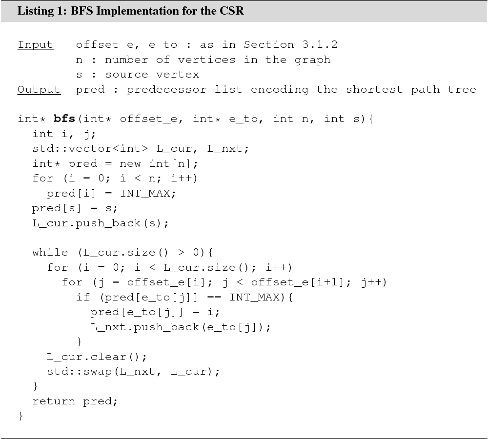
In an unweighted graph, BFS can be used to solve the shortest path problem, the single-source shortest path problem, and to extract the shortest path tree for an arbitrary source vertex. BFS takes linear time in the number of vertices and edges. An example implementation that solves the single-source shortest path problem for a graph stored in the CSR is shown in Listing 1. To solve the shortest path problem, the algorithm should be modified to terminate as soon as the destination vertex is found.
The algorithm maintains an array pred of size ![]() to keep track of vertices
that have already been explored, and to store a predecessor list that encodes
the shortest path tree or the shortest path. At the beginning of the algorithm,
each field in pred is initialized to a special value. If an arbitrary vertex
to keep track of vertices
that have already been explored, and to store a predecessor list that encodes
the shortest path tree or the shortest path. At the beginning of the algorithm,
each field in pred is initialized to a special value. If an arbitrary vertex ![]() is not reachable from the
source vertex, pred[v] still holds the special value when the
algorithm terminates. Otherwise, pred[v] holds the identifier of a
vertex on the next lower level to which
is not reachable from the
source vertex, pred[v] still holds the special value when the
algorithm terminates. Otherwise, pred[v] holds the identifier of a
vertex on the next lower level to which ![]() is adjacent. For the source vertex, pred[s]
is adjacent. For the source vertex, pred[s]![]() . To extract
only the length of the shortest path, or if BFS is merely used for traversing
the graph in breadth-first order, pred can be implemented as
a bit array.
. To extract
only the length of the shortest path, or if BFS is merely used for traversing
the graph in breadth-first order, pred can be implemented as
a bit array.
In edge-weighted graphs with non-negative
edge weights, shortest paths can be found with Dijkstra’s algorithm [5]. Dijkstra’s
algorithm is similar to BFS. It uses a priority queue to store vertices in the
neighborhood of already explored vertices in non-decreasing order of path
lengths from the source vertex. In every iteration, the head of the priority
queue is removed and the corresponding vertex explored. The running time of
Dijkstra’s algorithm is ![]() if an appropriate
data structure is used for the priority queue. A Fibonacci heap [7] is often
suggested, as it supports amortized constant time insertions, and logarithmic
time delete-minimum operations.
if an appropriate
data structure is used for the priority queue. A Fibonacci heap [7] is often
suggested, as it supports amortized constant time insertions, and logarithmic
time delete-minimum operations.
If some edges have a negative edge-weight,
the Bellman-–Ford algorithm [6, 3] can be used for solving the shortest path
problem. It takes time ![]() . Notice that in such graphs,
infinite paths may have an infinite negative weight.
. Notice that in such graphs,
infinite paths may have an infinite negative weight.
BFS can solve the example query put forth in the introduction to this section. The algorithm runs in linear time if vertex access takes constant time:
• For each ![]() , if the label of
, if the label of ![]() indicates that the paper was authored by Paul
Erdös and published in 1960, include
indicates that the paper was authored by Paul
Erdös and published in 1960, include ![]() in set
in set ![]() .
.
• Every ![]() is a source vertex. Initialize BFS by setting
pred[v]
is a source vertex. Initialize BFS by setting
pred[v]![]() and pushing
and pushing ![]() on L_cur for all
on L_cur for all ![]() . Start the search.
. Start the search.
• Terminate the search when a vertex ![]() is found where the label
indicates that it has been published by four researchers affiliated to the University
of Oxford.
is found where the label
indicates that it has been published by four researchers affiliated to the University
of Oxford.
• Follow the predecessor list pred backwards from ![]() until pred[v]
until pred[v]![]() . Print the
titles of the papers along the way.
. Print the
titles of the papers along the way.
3.2.2 Depth-First Search
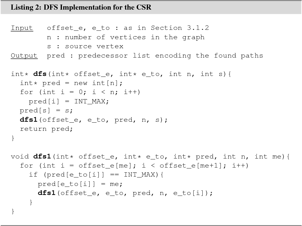
Depth-first search (DFS) can be viewed as the conservative counterpart of BFS. While BFS always explores all of the neighborhood of every vertex it reaches, DFS carefully steps ahead one vertex per level, returning to a previously visited vertex before exploring a new area of the graph.
A recursive C++ algorithm that implements
DFS for a graph stored in the CSR is shown in Listing 2. Just like the BFS
algorithm, the DFS algorithm maintains an array pred of
size ![]() to keep track of already explored
vertices and to encode the identified paths. Just like BFS, DFS runs in linear
time.
to keep track of already explored
vertices and to encode the identified paths. Just like BFS, DFS runs in linear
time.
DFS navigates as fast as possible as deep
as possible into the graph. Whenever it discovers an unexplored vertex ![]() , DFS starts scanning
, DFS starts scanning ![]() for the next unexplored vertex. When
the first such vertex,
for the next unexplored vertex. When
the first such vertex, ![]() ,
is found, it halts the scan of
,
is found, it halts the scan of ![]() and starts a scan
of
and starts a scan
of ![]() . The scan of
. The scan of ![]() is
not continued until every vertex that is reachable from
is
not continued until every vertex that is reachable from ![]() by passing only through unexplored vertices
has been explored.
by passing only through unexplored vertices
has been explored.
The figure below shows at which levels the vertices of an example graph are explored in BFS and DFS. The leftmost vertex is the source vertex in both algorithms. The list on the right side of each graph shows the order in which vertices at different levels are visited. The graph for DFS can be shown differently if the order in which vertices are selected from the neighborhood sets is different. The graph for BFS must look as it is shown.

DFS is useful for problems that involve
information encoded in the structure of the graph. Consider a directed graph
that encodes stock holdings among companies: Vertices represent companies,
edges represent holdings. If company ![]() is invested in company
is invested in company ![]() , the graph contains an edge
, the graph contains an edge ![]() , labeled with the relative amount of
stock held. DFS can be used to create from the graph an organized list of
direct and indirect influences of a given company .
, labeled with the relative amount of
stock held. DFS can be used to create from the graph an organized list of
direct and indirect influences of a given company .
The DFS algorithm shown in Listing 2 has to be modified for this purpose. Consider a situation in which a company holds stock of two companies, which are themselves invested in the same fourth company. In the current algorithm, the fourth company is ignored when it is discovered for a second time. For the algorithm not to ignore already explored vertices, the condition ‘if (pred[e_to[i]] == INT_MAX)’ has to be removed from function dfs1().
Unfortunately, if a vertex ![]() is visited for a second time, pred[v] is overwritten and information of (potentially several) previously
discovered paths is destroyed. The simplest remedy is to produce the desired
list as the search runs. This makes pred obsolete.
is visited for a second time, pred[v] is overwritten and information of (potentially several) previously
discovered paths is destroyed. The simplest remedy is to produce the desired
list as the search runs. This makes pred obsolete.
The output row for vertex e_to[i] can be generated just before the recursive call. The figure below
shows how the influences list could look like for an example graph. Company ![]() is the source company.
is the source company.

The company names are indented by the
levels at which they are visited. To achieve this, an additional argument int level has to be included with function dfs1(). level+1 is passed into the recursive call. Notice how companies ![]() ,
, ![]() , and
, and ![]() appear multiple times and with different
levels in the list.
appear multiple times and with different
levels in the list.
To add column ‘Influence’ to the output, two additional arguments have to be included with function dfs1(): float* e_w and float cur_perc. The vector e_w holds the edge labels (i.e., percentage holdings), cur_perc holds the influence of the source company on company me through the path that is currently being explored. The result of cur_perc*e_w[e_to[i]] is appended to each output row and is passed as cur_perc into the recursive call.
The box on the right shows the total
influence of company ![]() on
the other companies. The percentages are the sums of the respective percentages
in the ‘Influence’ column.
on
the other companies. The percentages are the sums of the respective percentages
in the ‘Influence’ column.
What if cross holdings existed, or if
company ![]() was invested
in company
was invested
in company ![]() ? Put
differently, what if cycles existed in the graph? The current algorithm would
fall into an infinite recursion, ultimately exhausting the memory stack or
overflowing the output device. The algorithm needs to be extended with a
mechanism that detects if a vertex that is already part of the path that is
currently being explored is about to be visited again.
? Put
differently, what if cycles existed in the graph? The current algorithm would
fall into an infinite recursion, ultimately exhausting the memory stack or
overflowing the output device. The algorithm needs to be extended with a
mechanism that detects if a vertex that is already part of the path that is
currently being explored is about to be visited again.
The simplest solution is a boolean vector active of size ![]() . Each field is initialized
to false. Before dfs1() enters into the for loop, active[me] is set to true. Just
before dfs1() returns, active[me] is reset to false. Where previously ‘if (pred[e_to[i]] == INT_MAX)’
limited the search, a new condition ‘if (active[e_to[i]] == false)’ is added. The modification ensures that no two instances of dfs1() with the same vertex in me can ever be active at
the same time. Optionally, an additional output column may indicate at which
vertices a cycle has been detected and skipped.
. Each field is initialized
to false. Before dfs1() enters into the for loop, active[me] is set to true. Just
before dfs1() returns, active[me] is reset to false. Where previously ‘if (pred[e_to[i]] == INT_MAX)’
limited the search, a new condition ‘if (active[e_to[i]] == false)’ is added. The modification ensures that no two instances of dfs1() with the same vertex in me can ever be active at
the same time. Optionally, an additional output column may indicate at which
vertices a cycle has been detected and skipped.