6  G-Store Storage Algorithm

6.1  Objective and Overview

G-Store puts the proposed desiderata into action. Following desideratum (1), G-Store stores the labels and edges of each vertex together. G-Store uses an efficient encoding system, separating edges to vertices in the same block from edges to vertices in a different block. Desiderata (2), (3), and (4) are realized through a multilevel algorithm. The objective of the algorithm is to find an approximate solution to the following problem:

where , , and  are parameters. Multilevel algorithms have previously been applied to the graph partitioning problem and the minimum linear arrangement problem. G-Store’s storage algorithm may well be viewed as an attempt to solve a combination of difficult versions of these problems.

Figure 8 illustrates the algorithm. The input graph is defined in a plain text file. Together with the schema definition, the text file is used to create a main memory representation of the input graph. This graph is coarsened until each of its connected components consists of a single vertex. Finding a -minimizing partitioning for the coarsest graph is a simple task. Iteratively, the coarsening steps are undone. In each iteration, the partitioning for the coarser graph is projected to the next finer graph, and refined. The partitioning for the finest graph is used to derive a placement of the input graph into consecutive blocks on the disk.

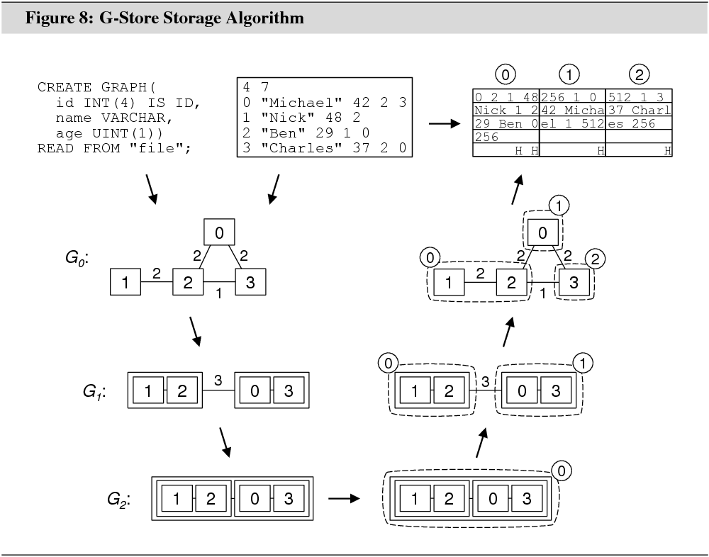
Throughout this section, we use  to denote the input graph defined in the text file. We use  to denote the graph at coarsening level . Each graph  is undirected and both vertex-weighted and edge-weighted (vertex weights are not shown in Figure 8). We use  and  to denote weights. We let  for an arbitrary  be the expected number of bytes that the vertices from  that are represented in  will use on the disk. We let  for an arbitrary  be the number of edges from  that connect a vertex represented in  with a vertex represented in .

We use  to denote a surjective function that maps the vertices in the graph at level  to partitions.  is not known. We use  to denote the set , and  to denote the sum .

The multilevel storage algorithm can be broken down into smaller algorithms. The coarsening algorithm (Section 6.3) first derives  for all levels. The turn-around algorithm (Section 6.4) then derives  for the coarsest graph. The uncoarsening algorithm (Section 6.5) derives  for the remaining levels. All algorithms have been designed to reduce  at each level. There is no strict constraint on the weight of a partition. However, the algorithms implement various heuristics to push  for all  for each level  below a bound that changes proportional to . The finalization algorithm (Section 6.6) ensures that  does not violate  for any .

6.2  Memory and Graph Representation

Implementation in read_input.cpp and move_to_disk.cpp.

The multilevel storage algorithm uses the compact storage format (see Section 3.1.2) to represent the graphs at the various coarsening levels in main memory. Each graph stores a pointer to the next finer and next coarser graph, much like a doubly-linked list. During coarsening and uncoarsening, the algorithm works on at most two graphs concurrently. If the algorithm runs out of memory at any time, it attempts to move a graph that is not currently used to a temporary location on the disk. It is read into memory again when it is needed.

The memory bottleneck is the coarsening from  to . These are the two largest graphs and if the algorithm runs out of memory, there is no graph that could be moved to the disk. In the next version of G-Store, it will be possible to run the storage algorithm on a part of the input graph if the entire graph cannot be represented in memory.

 is created directly from . The schema definition instructs the algorithm how to parse the text file that defines . Loops and parallel edges in  are ignored. Directed edges in  are converted to undirected edges in .  for each  is either one or two. It is one if the corresponding edge in  is directed, two if it is undirected.

 for each  is the expected number of bytes that the encoding of the corresponding vertex in  will use on the disk. A variable length character string in a vertex label, for instance, is accounted for with one byte per character, plus two bytes for a block-internal pointer. ’s edges are accounted for with four bytes per edge (based on  and ignoring loops and parallel edges). The actual size of each edge is not known until a partitioning has been derived. More details are given in Sections 6.7 and 7.2. In general,  is as least as large as the actual number of bytes.

6.3  Coarsening

Implementation in ml_coarsen.cpp.

G-Store’s coarsening algorithm is a variant of heavy edge matching (HEM), a greedy heuristic introduced in [13]. HEM is used in many multilevel graph partitioning algorithms and is implemented in both Metis version 4.0 (default coarsening method), and Chaco version 2.0 (optional, set via parameter MATCH_TYPE). HEM creates  from  as follows:

•    Set all vertices in  as ‘unmatched’. The vertices in  are visited in random order. Let  be the next vertex.

•    If  is matched, continue. Else, find an edge  such that  is unmatched and  is as high as possible. If no edge is found, continue. Else, set  and  as ‘matched’ and continue.

•    After all vertices have been visited, each unmatched vertex and each pair of matched vertices is mapped to one vertex in . Unmatched vertices keep their weight, matched vertices add up their weight.  is created from  by converting each edge to match the mapping to vertices in . Edges that would be loops in  are discarded. A set of edges that would be parallel in  is combined into a single edge that carries the weight of the set.

Since HEM prefers edges with a large weight during matching, and since loops in  are discarded, HEM tends to yield graphs with a comparably low total edge weight. This increases the probability that a partitioning for  with a lower cost  can later be found [12], maybe also with a lower cost .

In multilevel partitioning algorithms, coarsening is usually stopped as soon as  falls below a given value. In Metis, this value is set with hard code to . This choice is a further indication that Metis has not been designed for problems where the number of partitions, , is large.

G-Store’s algorithm keeps coarsening until . When coarsening is stopped, there will be one vertex in  for each connected component in .

Let us define . In traditional HEM,  tends to decrease with increasing . This is due to the emergence of “hub and spoke vertices” after repeated coarsening. Hub vertices are characterized by a very high degree and a large number of spoke vertices in their neighborhood. Spoke vertices are characterized by a very low degree and a hub vertex in their neighborhood. In traditional HEM, each hub vertex can be matched with only one other vertex in each iteration, leaving a large number of spoke vertices unmatched.

G-Store modifies HEM as follows: Two additional parameters are introduced,  and .  is the number of vertices that a vertex in  can be matched with in each iteration.  is the maximum weight of a vertex in .  is initialized to two,  to . After each iteration:

•    If  and :

–   If , set .

–   Else, set  and .

•    If  and , increment .

6.4  Turn-Around

Implementation in ml_turn_around.cpp.

Let  be the coarsest graph. Since , , regardless of , , , and .

The turn-around algorithm sets  to assign an individual partition number  to each  if . The remaining vertices can be assigned the same partition number  so long as .

6.5  Uncoarsening

Implementation in ml_uncoarsen.cpp, ml_project.cpp, ml_reorder.cpp, and ml_refine.cpp.

Each iteration of the uncoarsening algorithm takes , , and  as input and returns . Each iteration can be broken down into three smaller algorithms: projection, reordering, and refinement. Projection derives a first attempt of . Reordering and refinement modify this function; reordering by swapping partitions, refinement by reassigning individual vertices to other partitions and by clearing out entire partitions.

Before we describe the algorithms, we need to define additional notation: In each iteration, let the weight threshold  be the result of , where  is the average of all s that have been observed during coarsening.

We define the tension for an arbitrary vertex  to be the sum . The tension for a partition is the sum of the tensions of its vertices.

We define the modified tension for  to be the sum , where  are the vertices that  and  have been mapped to during coarsening.  is not needed to calculate the modified tension for a vertex in .

Finally, let  be a function that returns for a set  of vertices from  the set of vertices from  that have been mapped to any vertex in  during coarsening.

The projection algorithm derives a first attempt of . After the algorithm returns,  and  are no longer needed and deleted from memory.

The algorithm steps through the individual sets  one by one, starting at . Let integer variable  be initialized to 0.

•    If  = 1 or if , set  for all , increment  and , and continue.

•    Else, find and store the modified tension for all vertices in . Set vertex  () to be the vertex with the lowest (highest) modified tension. Set all vertices in  to ‘unassigned’, except for  and . Let integer variables  and  be initialized to  and , respectively, where .

•    and  are the roots of two trees. Iteratively, either the left tree (root ) or the right tree (root ) is grown, depending on which has the lower total vertex weight. A vertex can be added to a tree if it is yet unassigned, is connected to the tree, and has the lowest modified tension (left tree) or the highest modified tension (right tree) among the vertices that are connected to the tree.

•    Suppose the left (right) tree is grown, and suppose  is chosen to grow the tree. The next steps are:

(a) Set  (). Set  as ‘assigned’.

(b) If , increment  (decrement ).

(c) For each , subtract (add)  from (to) the stored modified tension.

•    After all vertices in  have been assigned to a partition in this way, the gap between  and  is closed: For each , set , where parameter  is 2 if , 1 if either  or , and 0 otherwise. Notice that one partition always contains vertices found through both the left or the right tree.

Finally, set , increment , and continue.

While running, the projection algorithm marks each partition of  with a boolean flag. A partition created under the first bullet point is marked true. A partition created under the tree growing algorithm is marked false if it is created through the left tree, and true if it is created through the right tree. The middle partition is marked false.

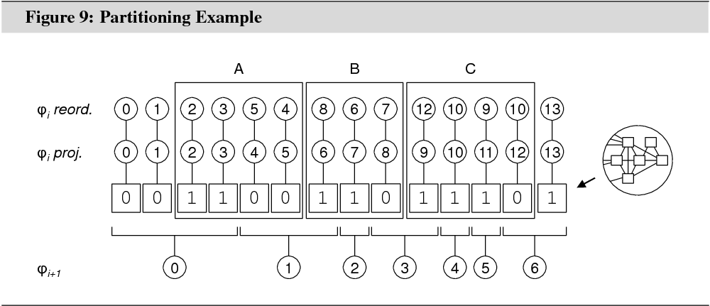
Figure 9 illustrates the states of the flags in an example with 7 partitions for  and 14 partitions for . A false flag is shown as 0, a true flag as 1. The row ‘’ shows the partitioning for . The row ‘’ shows a possible partitioning for  after projection. The row ‘’ shows a possible partitioning for  after reordering (see below).

The reordering algorithm attempts to reduce  through the swapping of partitions.  and  do not change during reordering.

Notice in Figure 9 how  after projection is bound to the partition borders in the coarser graph. Put differently, if for any , , then , , . The reordering algorithm breaks the borders.

The projection algorithm already tried to derive  in a way that reduced . It used modified tension, however, which is less expressive than tension. Now that a first attempt of  is available, the tension measure can be used to further refine it.

We illustrate the significance of tension in a simple example. Suppose that  for an arbitrary vertex , and suppose , , , , and . In this setup, the cost  incurred by vertex  is 20, and the tension on vertex  is . Figuratively, there is a force pulling on  from the left. It is easy to see that cost  can be reduced by moving  to a partition in the range [5..10). For instance, if  is set to ,  decreases to 16. An improvement of 4.

The example can be written for partitions as well:  would be set , and  and  would be sets  and .  would be , and so on. Moving a partition is more difficult, as setting  for all  would create a gap in the partition numbering. There are two solutions: One is to shift all partitions with a number greater than 10 left by one, the other is to shift partitions 8 and 9 right by one. The disadvantage of the former is that partition 8 might become very large. The disadvantage of the latter is that moving partitions 8 and 9 adds complexity as the effect of their move has to be taken into account when determining if moving partition 10 is beneficial.

The reordering algorithm identifies opportunities in the partitioning structure, where swapping two adjacent partitions decreases . Repeated swapping can move a partition by more than one position.

The algorithm steps through groups of partitions based on the boolean flags that were set in the projection algorithm. A group is defined as a sequence of true-flagged partitions followed by a sequence of false-flagged partitions. Partitions may only be swapped within a group. As illustrated in figure 9, each group (, , and ) contains partitions that originated from at least two different partitions in the coarser graph. This makes a certain degree of mobility between the partitions possible.

The algorithm uses an updatable, array-based priority queue to hold the swap alternatives in the order of their impact on . Repeatedly, the most beneficial swap is executed and the priority values of the remaining swap alternatives updated. Through repeated swaps, one partition can move from one end of the group to the other. The algorithm continues with the next group as soon as the best swap alternative in the current group does not improve . The implementation of the priority queue can be found in structs.h.

The refinement algorithm tries to reduce  by reassigning individual vertices to other partitions. The algorithm is one of the most complex in G-Store, and can be fine-tuned in several ways. Some parameters can only be modified in the code, others through G-Store’s parameter interface (see Chapter 7).

Five parameters can be set through the parameter interface: alpha, beta, gamma, runs_a, and runs_b. The former three correspond to , , and  in . Their default values are 0.125, 1, and 8, respectively. The parameters control the relative importance of the cost functions during refinement. In general, the parameters should be centered around 1.

runs_a sets the number of iterations of the refinement algorithm for the 8 finest levels (). runs_b sets the number of iterations for the remaining levels. Their default values are 3 and 1, respectively. Lower values reduce computation time, higher values can yield a better partitioning.

Let  count the number of iterations, starting at 0. In each iteration, the refinement algorithm randomly steps through the sets  for all . Let  be the next set.

•    The algorithm creates a two-dimensional matrix , where . Every entry  is a 3-tuple  that contains the negative of the change in costs , , and  if vertex  is moved to the partition with number .

•    After the matrix has been created and filled, the algorithm calculates a score for each entry:

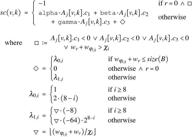
Repeatedly, the entry with the highest score is found. Suppose  was that entry. Then, if

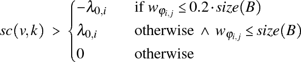
evaluates to true, vertex  is moved to partition , and all entries in  that are affected by the move are updated. Otherwise, the algorithm continues with the next .

Notice how scoring differentiates between  and , and between  and . For , an entry can only have a non-negative score if all , , and  are non-negative. Compared with , this yields a more selective group of vertices that are moved.

 is used as a reward for moving a vertex to a partition whose weight plus the weight of that vertex is not larger than . If the weight of partition  is itself not larger than , the reward is canceled out by a higher threshold to move.

If the weight of partition  drops to or below , the algorithm changes the threshold to move to the negative of  to facilitate moving for the remaining vertices. When partition  is cleared of vertices, all partitions with a number greater than  are shifted left by one to close the gap in the numbering.

 is used as a penalty for moves that increase the weight of the target partition beyond . The penalty depends on the size of the target partition and . For , where , the minimum penalty is .

6.6  Finalization

Implementation in finalize.cpp.

The finalization algorithm projects  to  and takes care of any partition  where . Recall from Section 6.2 that  for each  is an approximation of the actual number of bytes that the representation of the corresponding vertex in  will use on the disk. The finalization algorithm works with the actual number of bytes (see next section).

The treatment of partitions that are too large to fit in a block is based on the change in costs  and , with priority being given to the latter. The algorithm is similarly complex as the refinement algorithm and will not be discussed in detail here. We refer the interested reader to finalize.cpp.

6.7  Block Structure

Implementation in block.cpp.

Every block consists of a fixed size area, followed by a data area, followed by a header area. Free space accumulates between the data area and the header area. The fixed size area stores information about the contents of a block and occupies  bytes.

Each vertex has an associated header that occupies number of VARCHAR labels in the schema definition) bytes. Each header in a block has a unique slot number. The header adjacent to the end of the block has slot number 0. The header adjacent to the header in slot 0 has slot number 1, and so on. The slot numbers determine the order of vertices in the data area. The data for the vertex whose header is in slot 0 is stored adjacent to the fixed size area. If the block is completely full, the header with the highest slot number is stored adjacent to its vertex data.

Vertex data is stored in the following order: fixed size labels, VARCHAR labels, edges to vertices in the same block (“internal edges”), edges to vertices in a different block (“external edges”). A header consists of two-byte pointers into the data area. Without a VARCHAR label, the first pointer marks the beginning of the fixed size labels, the second marks the beginning of the external edges list, and the third marks the end of the external edges list. The internal edges list begins right after the fixed length labels and ends right before the beginning of the external edges list.

Internal edges are encoded as header slot numbers and use either one or two bytes of storage. Internal edges have the same size in all blocks. The size is decided in the finalization algorithm. If less than five in thousand blocks contain more than 256 vertices, one byte is used, otherwise two bytes are used. With one-byte internal edges, every block can store up to 256 vertices. With two-byte internal edges, every block can store up to 65,536 vertices. The finalization algorithm moves vertices out of blocks that contain too many vertices. The finalization algorithm also sets a number of function pointers to avoid having to repeatedly test for the size of internal edges.

External edges are encoded as global vertex identifiers (GIDs). A GID is an unsigned four-byte integer that encodes a block number and a header slot number. G-Store does not need an index. A GID is sufficient to find a vertex on the disk in constant time.

Each vertex has a unique GID: Let  be the largest number of vertices stored in any block. Let  be , and let  be . The  lowest bits of any GID are used to encode the header slot, the remaining bits are used to encode the block number. Thanks to C++’s bitwise operators (&, »), both numbers can be extracted efficiently.

For instance, if , then  and . In this setup, the vertex with GID 648,731 is stored in block 1267, header slot 27:

Both the internal edges lists and the external edges lists are sorted in increasing order. G-Store’s query engine exploits this in various ways. For instance, by implementing cycle detection with binary search.

G-Store creates three files in its working directory that might be of interest. These files can be deleted.

•    _gidmap.g stores the mapping from  to GIDs. Line  contains the GID for vertex .

•    _parts.g stores function . Line  contains the partition number for vertex . Based on this file, G-Store can recreate the disk representation for the input graph without having to rerun the storage algorithm. See Section 7.2).

•    stats.g stores various statistics of the placement, both per block and on an aggregated level.